Yield, Energy and Throughput Optimization

Executive Summary

There are many different approaches to process improvement such as Six Sigma, Lean Manufacturing, Lean Six Sigma, Total Quality Management (TQM), Toyota System Production/Just-in-time, and the Theory of Constraints. Each of these methodologies has its strengths and weaknesses. For example, Six Sigma has a history of working well to make incremental improvements using its proven DMAIC methodology (Define, Measure, Analyze, Improve, Control). However, it does not do very well finding breakthrough performance opportunities and it usually requires broader changes to one or more elements of the business model. Before diving into a problem with any methodology, however, it is usually best to get an overview of the issue at hand and an understanding of skill set required to address it.

Understanding the Situation

In the world of manufacturing, three of the most important factors to consider include energy used in production, yield (or ratio of non-defective items produced compared to the total items manufactured), and throughput (the amount of product produced). All these factors play a key role in accomplishing your business objectives, so understanding how they impact each other and how to strike the perfect mix between all of them is very important.

A simple example from linear algebra illustrates the power of using big data solutions to drive improved production rates. We can write the equation of any straight line, called a linear equation, as: y = mx + b, where m is the slope of the line and b is the y-intercept. If we consider that y is the thing that we are trying to optimize and x is our production rate, then we may break this point slope formula into two different entities:

1. mx – this is the portion of yield or energy that is dependent on the production rate
2. b – this is the portion of yield or energy that is independent on the production rate

Why is this important? There are two reasons: a) experience has shown that there are usually different skill sets required to solve each portion and b) to determine which portion has the greater opportunity for improvement. For instance, in a process plant, improving mx usually requires process control tuning and optimization. On the other hand, b frequently requires some form of system change to improve, which may require a capital investment.

We can now take all the available information on y (yield or energy) and x (production rate) and run a simple linear regression to determine m and b. Once we determine m and b, we can determine which portion of the relationship has the greater effect. However, y = mx + b is a simplified version of the more general y = m1x1 + m2x2 + m3x3 + m4x4 +…+ b. Production rate may not be the only factor affecting energy usage so we must look at it in a larger context. Therefore, we will consider y to be total energy usage and (x1, x2, x3, x4, …) are variables such as production rate, labor, etc.

To achieve the business objectives, we need to consider the following:

• For which aspect of energy we are optimizing? Are we minimizing energy usage or minimizing energy cost and what are their constraints Simplistically, we can minimize energy by shutting down the plant entirely but that is usually not economically beneficial. This means that we must observe at least some production constraints.

• Are we minimizing energy usage, energy cost, maximizing production or are we driving for a balance across these metrics? To improve the current process, we need to understand and align with the enterprise level objectives.

• What are the drivers of the objective? At Kaizen Analytix, we leverage our Kaizen DriverSelector to find significant drivers on our desired objective for the system.

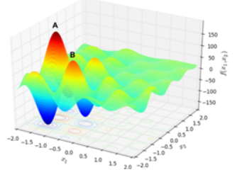
Once the questions above have been answered, the next step is to establish the system objective and significant drivers as a mathematical function. We leverage our KaizenValueAccelerators™ library of prebuilt analytics components to incorporate competing metrics within an objective, understand the impact of constraints, evaluate hard as well as soft constraints and drive actionable recommendations in a short period. In real-world problems, objectives usually have non-linear relationships. Our analytical dashboards and metrics identify whether current operation is closer to a global optimization or a local optimization. Our KaizenValueAccelerators™ are flexible enough to support commercial solvers like CPLEX, Gurobi or Open Source versions like Python – PuLP or SciPy.

Accounting for Variability - The Funnel Experiment

Of course, this is not the only data we need to examine. We also need to understand the variability of the system. Dr. W. Edwards Deming devised a simple experiment to show how important it is to know the system variability called The Funnel Experiment. This experiment describes the adverse effects of making changes to a process without first making a careful study of the possible causes of the variation in that process. Rather than improving the process, Deming referred to it as “tampering” with the process.

The first goal of any improvement process is to understand the natural variability of the system and work toward minimizing that. Once the variability is at an acceptable level, we can affect changes to improve the system. Looking at the control chart in Figure 1, we would say that it represents a system in control. There is random variation around a mean value. The upper and lower control limits (UCL and LCL) are usually set at ±3σ (standard deviations) from the mean. There is also sometimes a specification limit (USL) that the product or process may not exceed. This specification may be a product purity specification or even a compliance limit such as odor threshold.

Figure 1

If we alter the system and do nothing to minimize the variation, we may create problems for ourselves. Suppose it is economically advantageous to move the average closer to the specification limit. We are going to do this without worrying about the variability. Here is what the new control chart may look like:

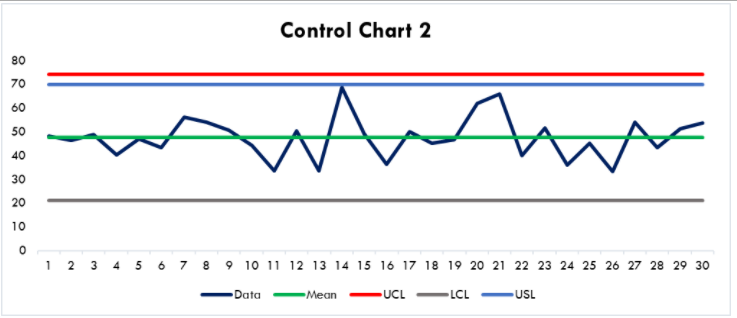
Figure 2

Now our specification limit is inside our control limits. Since the control limits are set at 3σ, this means, statistically, about 1 in 370 times we will fail to meet this specification. We term this an incapable system. This may be acceptable or just a minor nuisance to the facility. At the other end of the spectrum, if this is a compliance limit, it might result in having to report to regulatory authorities such as the EPA or state environmental agency. Now let us see if there is another way to achieve our objective.

Suppose we work on the process and reduce the variability by 1σ. Now the control chart looks like Figure 3:

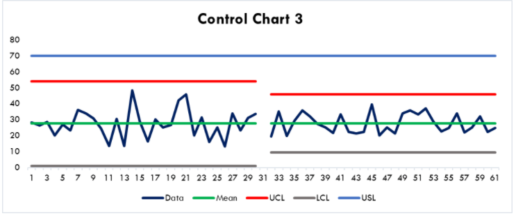
Figure 3

When we move the average closer to the specification limit now, we still have a capable system as shown in Figure 4:

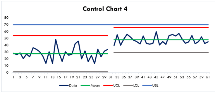
Figure 4

Once we understand the sources of variability and their effects, we can look for ways to improve the system. This is where data analytics can help. To accomplish this, we leverage our Kaizen ValueAccelerator™ library of prebuilt analytics components to rank the importance of variables in a regression or classification problem in a business reasonable way. This will tell us how important each variable is to the total outcome. The real power of data analytics is in its use over a broad spectrum of data. Not only can we look at the normal process variables of temperature, pressure, etc. but we can also add in non-continuous data such as scheduled shift number, day of the week, or even phase of the moon. This allows the analytics to find correlations in unlikely places or to uncover hidden plant issues. The big data solutions in Kaizen Analytix’s internal design and development process addresses the inherent variability in the system to avoid adoption risk and performance issues.

Success Stories
In one chemical industry application, the data analyst was studying an ethylene oxide unit and found that there was a correlation between a heat exchanger and the productivity of the reactor where there should not have been. It turned out that, unbeknownst to the operating staff, there was fouling in the feed cross exchanger and this led to the unexpected correlation. This fouling hindered production and reduced selectivity to the desired product (Hydrocarbon Processing, July, 2020). In another chemical industry example, product mix in an ethanolamines plant was the issue under study. This plant makes three products simultaneously, MEA (monoethanolamine), DEA (diethanolamine), and TEA (triethanolamine) in varying proportions. Using data analytics, the most important factors contributing to the selectivity of DEA were identified and selected an optimal production strategy that reduced the production rate of undesirable byproducts DEA and TEA by 66% (Hydrocarbon Processing, July, 2020).